How did we manage our BI datawarehouse migration?

Building a new data warehouse may seem like a herculean task - and, in a certain way, it is.
A pessimistic Analytics Engineer could say that creating and maintaining a clean pipeline is a never-ending task, no matter how much effort you put into it - almost sounding like Sisyphus rolling a boulder up a hill just to see it roll back down. That’s another valid and compelling point of view.

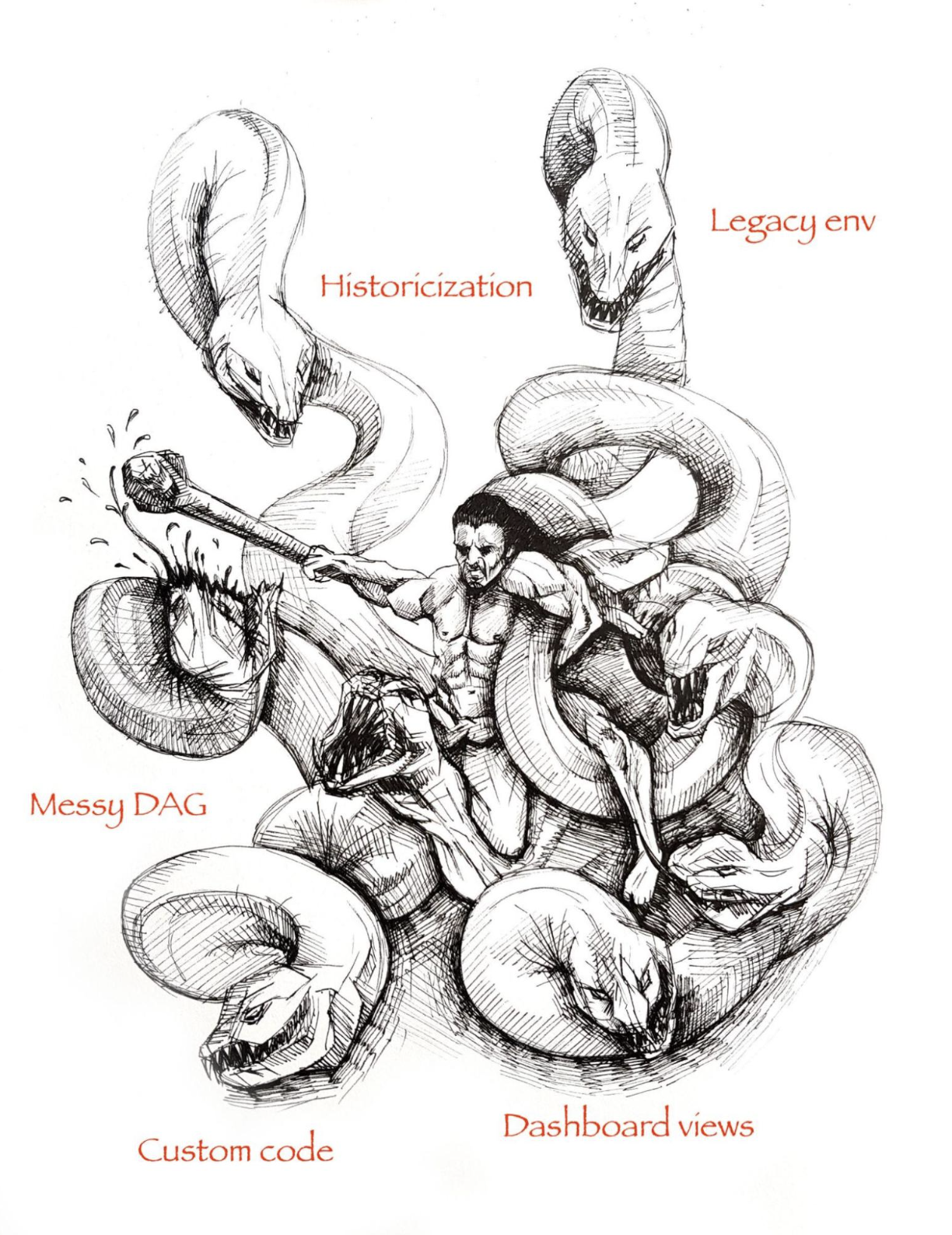
The goal of this article, however, is to show that, with the right resources and processes, there’s no need to be Hephaestus to create a pipeline that shares the same greatness of Poseidon’s Trident; that by choosing the right Hydra’s heads to cut, you will be able to fight the most worthy battles to give your team the most essential and impactful pieces of data; and that finally, one must imagine our Analytics Engineer Sisyphus happy with the progress made in each iteration to improve their warehouse, no matter how much work is still left for it to be perfect.

Ready to learn how we tamed this hydra? Equip your most robust helmet headset, sharpen your mind and take your healing potion (a coffee could do the job) to live this heroïc adventure with us.

Legacy environment limitations and issues

At Contentsquare, the Product Analytics team supports Product teams in taking data driven decisions regarding strategy and features improvements. This concretely translates into building dashboards & running analyses about usage. All of these data assets require having a robust and trustworthy data infrastructure that our Product Analytics team continuously builds and maintains.

Robust and trustworthy: two words that were far from characterizing our legacy data pipeline and that we raised as golden rules to build our new data warehouse. In this part, we will present our previous infrastructure’s key issues to further show how we solved them by building the new one.

DAG issues

Looking back a few months ago we were able to identify some of the pitfalls we went under since the team was created. This was what one of the main branches of our data pipeline looked like before the migration to the new pipeline

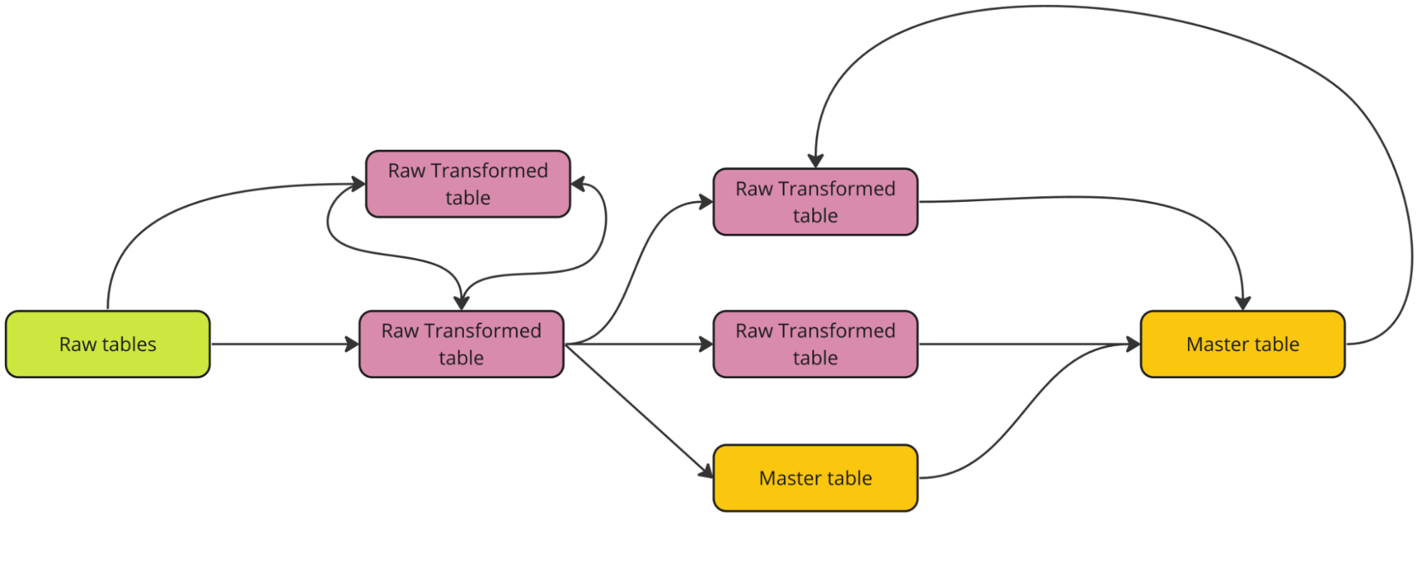
We had four schemas: three of them for the raw data and one of them for transformed data and here came the first three issues with this infrastructure:

1. Raw data schemas allowed data transformation from raw data, which was not raw anymore,
2. It is impossible to have only one transformation schema without opening the possibility for DAG loops and interdependence between assets and
3. Use case specific assets forced people to build redundant tables with the same kinds of data and transformations, due to an impossibility to use those for most of the use cases.

Those issues that seem pretty technical at first glance led to painful and concrete issues in analysts’ daily lives. When you transform raw data before ingesting it, anyone needing the same raw data as you for a different use case will have to repeat the same ingestion tasks prior to working on their own. Loops in your transformation layer prevent you from being able to easily create your whole pipeline from zero, which is sometimes needed because of disruption.

Finally, when you have two assets trying to reproduce the same logic, it is highly likely that people who created them will do it in a slightly different way, changing the logic or including/excluding one or another dimension/metric - leading to “multiple sources of truth” for a same metric or report, drastically affecting the trustworthiness of the team when interacting with stakeholders.

Custom Python code

To build this entire environment, the former Analytics members used mostly Python. It means that all the data extraction, transformation, and load steps were made with Python code. That is not a problem at all per se, however, some limitations turned it into a huge bottleneck for the whole team. There were almost no conventions or rules to create new code, so every new data source or transformation could be in a completely new code style, which made it very hard for other analysts to apprehend. Debugging or changing someone else’s code was then a lengthy and tedious process. More than that, Python was not something required to new joiners (because of a Product Analytics candidate shortage), which made it even more complicated to onboard new people in the new infrastructure.

Collaboration between analysts

When you do not have a structured data pipeline, things get worse with service disruptions and (the absence of) post-mortems. In our first data pipeline, we had a repository in GitHub in which every analyst and engineer was a contributor. Every change was done on a local branch and then pushed to the production branch. Pretty classic. So what was wrong then?

We did not have a safe environment to test our changes and new models. If someone wanted to test them extensively, they would have to go through a very manual process of creating a new temporary table with the changes, and do the same to all models that depended on that table. As you might imagine, it was done very rarely, which led to many bad changes being updated to production, causing assets to break and spending a lot of analysts’ time on debugging and fixing the issues. Peer reviews processes were not preventing anyone to run a code locally that was directly impacting our production environment (meaning all the tables and assets that analysts are querying on a daily basis).

Lack of historization

In our legacy environment, all data coming from external sources was ingested in a way that would overwrite the existing data and replace it with new data. In this scenario, getting a picture of today’s status and KPIs is possible, but looking into historical data becomes tricky.

Dimensional data - client or user information - is frequently updated: a user might have some access rights today and have them removed in some months, and a client might have had access to a feature 6 months ago but no longer does. In both cases, only the most updated data would matter in our legacy data warehouse, which prevented us from getting the right KPIs in some cases and simply made our data become wrong depending on the angle we looked at it. Answering the basic question: “what was the usage of accounts that churned last year?” was hard because these accounts did not appear anymore in our main tables.

Some key tables were historized in the legacy environment using Python custom code, but it was hard to scale this code to all tables in our environment.

Lack of code readability

Every analyst who has worked enough time in this position - one month should be enough in most cases - has already been asked the following question: “The data shown in this report seems wrong, could you check?”. Creating and maintaining dashboards are part of every analyst’s job, and these kinds of questions should be easy to answer if we want to build trust with stakeholders.

In our legacy environment, we used Python custom code to query our databases and create CSVs that would be sent to Google Cloud Storage and used in Data Studio as data sources. It means these data sources were not materialized: the only output of the scripts was a CSV sent to GCS. Thus the only way to get the exact data sent to a dashboard for debugging would be to ingest this CSV locally or to extract the query from the script and run it in your machine. Both options were very manual and time-consuming, and none effectively solved the issue of not being able to easily query the data sent to Analytics tools. Some data checks that should have been easy to perform were intricate and troublesome

Changes in raw data

Our team stands in Product. It means one of our responsibilities is to monitor the adoption of new releases on our software. An Engineering team is in charge of delivering these features, and to store information about them in a database (the “production database”). This database then feeds our own internal analytics system.

Problem: there are more than 300 people at Contentsquare Engineering team, spread across more than 25 units. It was impossible for a small team like ours to follow up manually on all the changes operated on the production database every week.

We could not follow up on changes manually, and our legacy environment… did not take care of it automatically for us either. We were not alerted of the differences between existing assets on our side and the raw data coming from the developers’ databases. Worse: when noticing a column had been deleted or renamed on developers’ end, we often had to go through a manual process of adding tables and columns to all dependent assets, or sometimes even recreate tables from scratch.

The legacy data environment used Amazon Redshift as a data warehouse, and Python custom code to ingest, transform and load data. As you might expect, custom code is very good at getting to the “It works! Let’s not touch it anymore” step, but can get quite messy without clear rules, conventions, or documentation.

It was probably the natural path for a growing Analytics team proving their worth and value to build things that way, and, most importantly, it worked! The team gained stakeholders’ trust, was able to deliver value, and shaped the company’s strategy with analyses, OKRs, and dashboards.

We thus needed to reach the next level: rethink our environment to absorb growing requests, scale and gain in data quality and robustness.

Reshaping our data warehouse

Structuring our transformation pipeline to fit our needs

When starting to build our new conceptual architecture we quickly realized that the available materials to correctly structure a transformation pipeline with dbt were not fitting the complexity of our requirements. We wanted to take the best of dbt guidelines and use them to our advantage, so we went ahead and built our own framework on top of this foundation.

Our different types of data and business use cases led us to adopt the final transformation pipeline described in the following schema.

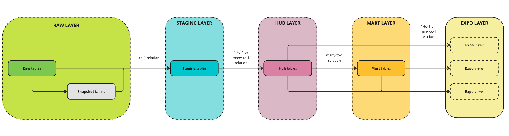
The first important thing to notice is that we switched from a previous infrastructure with no clear rules and loops to a clear sequential framework where each transformation is the output of the preceding layers. There is no asset in a given layer that is built from another asset of this same layer. Sticking to this design/principle was sometimes challenging and there were edge cases we managed to overcome but overall, it helped avoiding code duplication and maintaining a sequential architecture that’s consistent and easy to understand.

When splitting a transformation pipeline into coherent and useful layers, you need to be mindful to not adhere too much to one specific business need, so you answer them all.

Here are the main rules we defined to answer this challenge.

Raw Layer

The Raw Layer is made of tables that are copied from the different sources of data we have.
We then used the framework of Dimensional Modeling to distinguish between two cases of data:

• Facts data: they usually refer to events. In our specific case, all the pageviews and clicks data performed on our Product by clients are facts data.
  • Facts data will flow from the raw table (copied from the source data) directly to the staging models.
• Dimensions data: all the data that characterizes or describes a given object, user, order… For instance, we have data that describes each of the users that browse our tool (is it an employee? What is its company? etc).
  • Dimensions data will flow from the raw tables to snapshots tables where dbt allows us to record all the changes of these dimensions (if the company name of a user changes for instance). This way, all the historical changes of this data are stored before sending them to the staging layer.

Staging Layer

The Staging layer has a simple and unique goal: cleaning the data without doing any big transformation. We are here only doing columns renaming from the Raw layer, type casting and basics transformations like transforming a column from seconds to minutes for instance. The relationship between Raw and Staging is really a 1 to 1 relationship so there are no joins performed.

Hub Layer

The Hub layer is the layer where we perform more complex computations and combine different staging tables. We defined one main rule to avoid going in all directions when building hub tables: each Hub table must represent and concern only one entity.

Let’s take a concrete example to illustrate this rule:

• In our business, we deal with pageviews and so we have dimension data coming from different staging tables that describe these pageviews (for example pages names and categories).
• We also deal with clicks data and have dimension data that describes the elements that are clicked (for example zones names and categories).
• In this example we thus have 2 separate entities: pages dimensions data and zones dimensions data and so we will thus create 2 Hub tables and never create 1 unique Hub table that would mix the two different entities.

Mart Layer

The Mart layer is composed of the main tables we use on a daily basis. We made the choice of limiting the number of the tables inside this layer to benefit from the column oriented performance offered by our Snowflake warehouse. This allows us to have a simple and more readable layer that is designed to serve a vast range of use cases with very few tables: ultimately, we aim at serving 90% of our daily use cases only with a couple of tables.

The Mart tables are thus tables that will combine different entities from the Hub layer. In this paradigm our main most useful table is actually a table that regroups pageviews, clicks events (stored in arrays or JSONs) and dimensions columns (user names, account properties).

In a nutshell, Mart tables:

• Are built from different entities,
• Serve a wide range of use cases,
• Are limited in number and not redundant between themselves

As the Mart tables can be pretty big they are not designed to directly serve our dashboarding purpose. On top of that, dashboarding is really tied to specific use cases and we did not want at this stage to have an accumulation of tables for each specific use case: Mart tables are really here to serve the next layer (for dashboarding) and our daily analyst job of querying and crunching data.

Because of the complexity of our data we needed the preceding four layers of transformations to finally reach the point where we have all the assets to fill our needs: ad hoc export requests, exploratory analysis and dashboarding. In our data stack we use Tableau software for our dashboarding tasks and so we could have ended our transformation pipeline at the Mart layer and then call these tables through custom SQL queries inside Tableau. The huge drawback of this is that you don’t have a unique place where you can clearly see which query feeds which purpose (as you will have all the queries disseminated in the several Tableau workbooks your team builds). In this context whenever you need to change a KPI computation that affects different dashboards you will need to know which dashboard is concerned (and there is no way to know it apart from checking them all or asking each analyst of your team) and you will never have versioning.

This is why we went with a 5th layer that entirely serves our dashboarding needs. The Expo layer is only made of views that are custom to the use cases they fulfill. You can see a view as a source for our Tableau dashboards and each view is directly called inside Tableau without performing any additional custom query inside Tableau. This way we ensure that we keep track of every query that serves any dashboard inside the same dbt project and this makes it easier to share similar pieces of code between different views and change KPIs computations on several views at once if needed.

Finally, even if the full pipeline is composed of five layers, the advantage of our architecture is that we can clearly split its layers in terms of usage as depicted below.

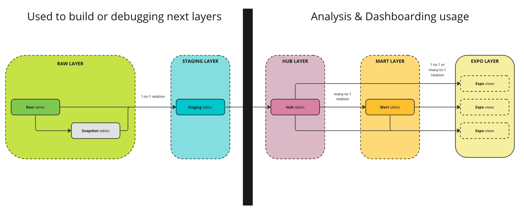
This allows us to have an even clearer view of our data warehouse based on the task we want to perform:

• Analytics engineering tasks (building new tables) will often require to open the raw and staging layers.
• Purely Analytical tasks will actually only require to focus on 2 to 3 layers of cleaned data without bothering with raw or staging data.

This is helpful when your team is made of analysts with different skill sets: the pure analytical analysts now will not bother with 5th but 2 to 3 layers of pipeline.

Historization: our DeLorean to uncover the past and drive the future

Wait A Minute, Doc. Are You Telling Me You Built A Time Machine… Out Of A DeLorean?

As previously stated, one of the main pain points our team was facing with the legacy infrastructure was that we were completely blind about the changes made on our dimensions data (the data that describes our users, objects etc). Our old DeLorean infrastructure was not well suited to easily keep track of historical changes until Doc (dbt) came out with its temporal convector: the snapshots dbt models.

What Snapshots models are

The vast majorities of our raw tables are of a SCD type 1. It means that whenever a change is made on values of a given entity the given row of this entity is UPDATED and we lose the past values. You will never be able to know what were the different characteristics the given entity had in the past in these raw tables: you can only know what the current value is.

The Snapshots tables in dbt allow us to track and keep the history of the changes that are made to the row of an input table (this is SCD type 2, i.e. you create a new row with the new values for this entity).

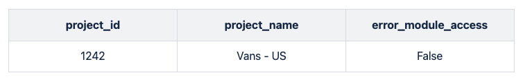
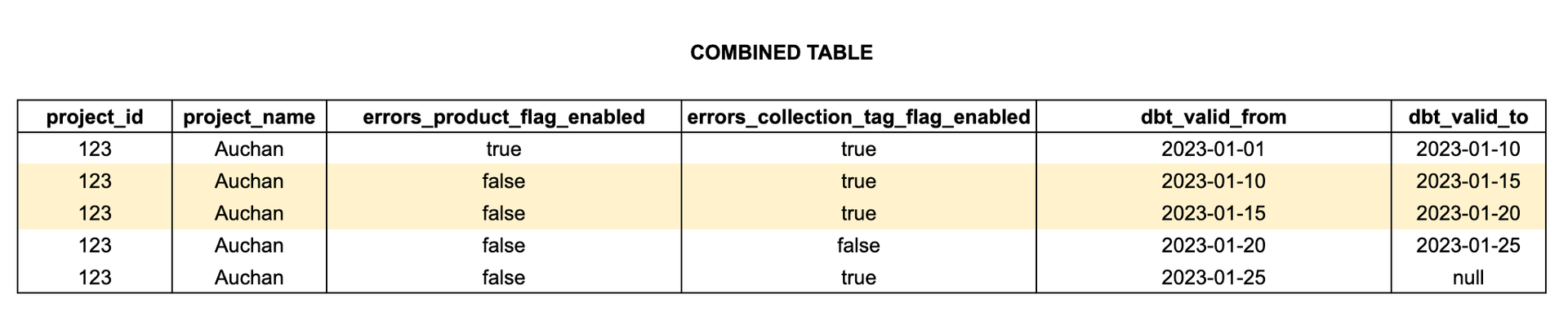
As a quick example to illustrate how Snapshots models work let’s imagine we have the following raw projects table

Now imagine that a Contentsquare employee is finally giving access to the Error Module during the day then if you query again the same table after this change you will get:

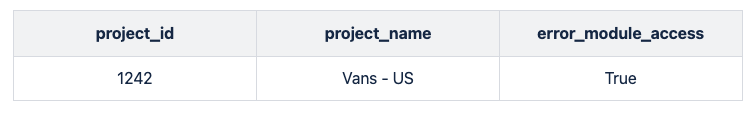
You are not able to know anymore that this project didn’t have access to the module during a period and you don’t know when this change happened.

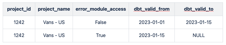
This is where dbt snapshots tables come along each day they compare the values which were valid so far to the current values of the input table. Our snapshot table will then actually looks like this:

Performing historical combinations

Joining two or several historized tables was not a trivial task because the dbt_valid_from and dbt_valid_to of the tables were often overlapping. To easily perform an historical join we built a Jinja macro that takes as input as many historized tables we want and gives the SQL code that performs the correct combination of these tables.

To illustrate how historical JOIN works let’s take a concrete example

Suppose we have the following two Dimension tables we want to JOIN

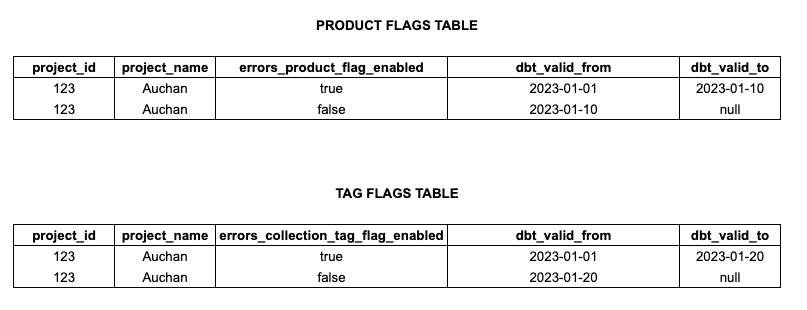
You can actually see that the validity period sometimes overlaps between the 2 tables and so we need to take that into account to combine these tables.

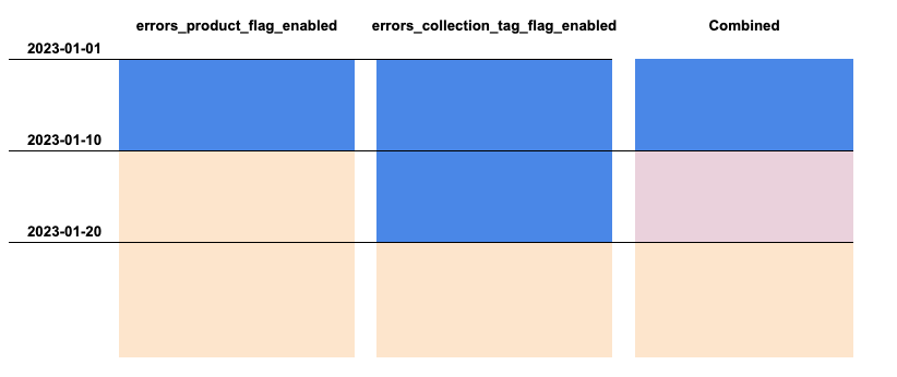
Blue color refers to the flag column being TRUE. Orange color refers to the flag column being FALSE.

So we do see that even if we have only 2 time periods in both tables then if we want to combine them it actually means having a 3rd period (the Red one) where we will have a mix of TRUE and FALSE.

Our Jinja macro builds the right SQL code to perform the correct combination so the output is:

Where we indeed see the 3 validity periods, which take the overlaps into account. Bear in mind that working with historized tables might not be that trivial when you want to perform combinations.

Historized data and the duplicates challenge

The following obstacle was that snapshot data were historized for all the columns of your table.

This means that whenever you select only a portion of the columns from your table you might face the issue of having multiple validity periods for identical lines. Creating clean tables that are built from historized joins of snapshots tables led us to build another tool again thanks to a Jinja macro that can easily be called to remove the duplicated lines and get a clean history.

To illustrate the duplicate challenge let’s take a concrete example

Suppose we have the following two Dimension tables we want to JOIN

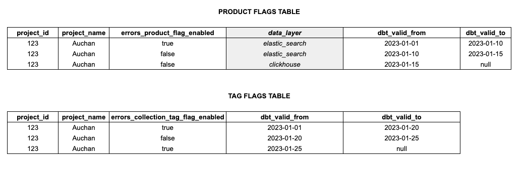
The gray column data_layer exists in the raw table but don’t want to have it in our final SELECT after the historical JOIN. However you can already see that this column has an impact on the validity periods because it changes over time.

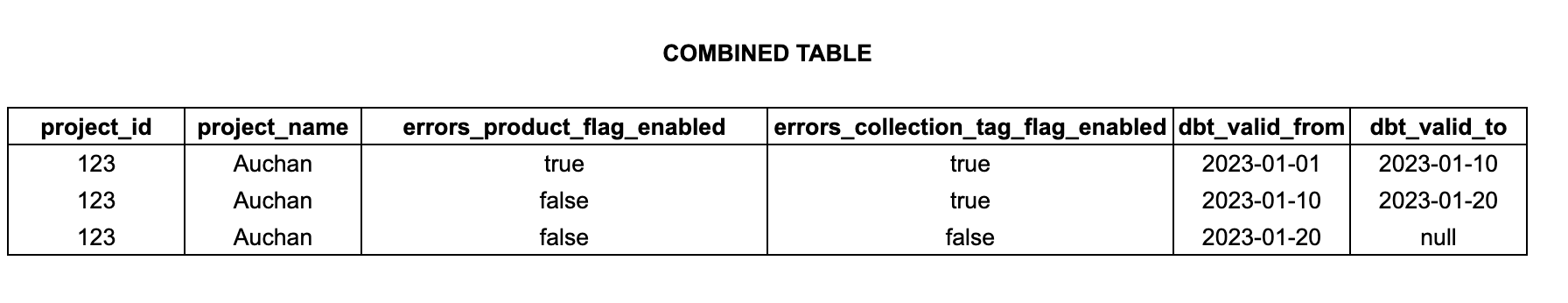
We join these two tables using our Jinja macro and only pick the columns we are interested in (= all of them except the gray column). The output of the combined tables will then be

This combined table has 2 rows (in yellow) that are actually exactly the same but have 2 validity periods that are actually continuous. We have 2 rows because under the hood there was this gray column that was changing during this period. But as we don’t select it, it can be weird and useless to keep these 2 rows rather than having a unique one with 1 unique validity period going from 2023-01-10 to 2023-01-20.

This is where we use the deduplication macro which will provide us with:

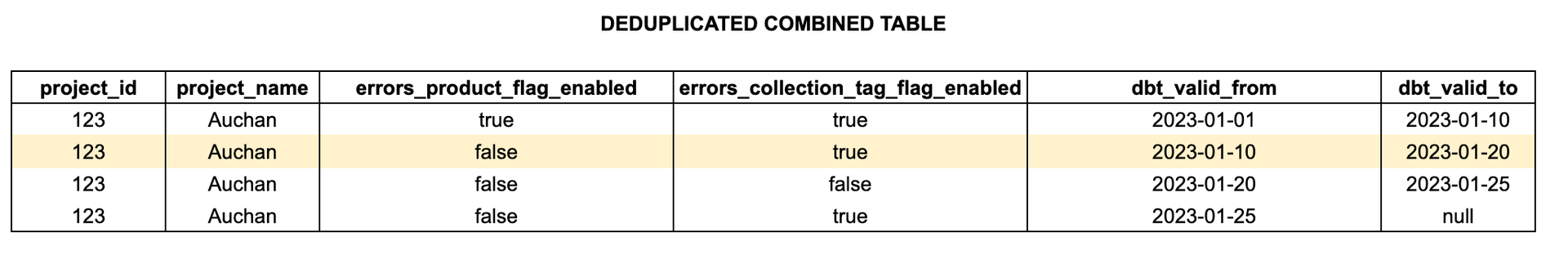
Where we indeed see the removed the duplicates and made the validity periods continuous as expected.

To sum up, dbt snapshots models and historized data is a must have to perform correct and deep analyses but to uncover correctly these functionalities you might need to build on top of them additional tools like we did to ease your team’s work.

Standardization and common rules

If you see our old infrastructure as the hydra and each of the limitations stated in our first section its several heads then cutting them was certainly necessary but not sufficient: it is well known that a hydra’s heads grow back when they are cut. You need to ensure that you don’t even let such a monster come alive. This is where standardized procedures and common rules come into play.

Setting Naming conventions to avoid confusion

This might sound trivial but when working with different analysts teams on a same data warehouse things can quickly become uncontrollable especially regarding fields and columns naming. Ensuring that we share the same column naming nomenclature was the very first step when building a cleaner infrastructure. The field renaming happens as soon as possible in the transformation pipeline in the Staging layer.

The sooner the better because first it reduces the number of analysts that might deal with fields naming: as stated in the previous section that presented our infrastructure only few analysts really act on modifying the Staging layer. Second because it ensures that all the analysts get the right naming of columns at the earliest level possible so that we don’t end up with table creation that differs from one analyst to another as everyone gets the correctly labeled data directly.

Naming of common assets should be fixed and done the earliest as possible inside your pipeline.

Building reusable code macro for our dbt infrastructure

To not let our data warehouse become a monster, we ensured every analyst could now call the same piece of code rather than coding filter conditions by themselves inside their own models.

As an example on our side we often use “valid” filters to only focus on pageviews made by our clients (removing pageviews done by our employees) and discarding test accounts. All these conditions are integrated in a Jinja macro that is then called by any model that needs these filters.

This reduces human errors (forgetting a necessary filter) and eases the modification you might want to perform as a team on these filters or computations. Do you want to change the definition of what a valid pageview is? Easy, you only need to change one piece of code inside the macro rather than changing dozens of files where these filters appear.

Building user defined functions for querying Snowflake data

Controlling human errors also relates to giving easy tools to your team to query complex data efficiently. Our infrastructure is based on Snowflake, which has arrays and JSON data types. These types are very useful in our case because it allows us to have very fine grained data without exploding this data into different tables.

However, Snowflake functions to query such data proved to be quickly limited for our use cases and so if we wanted to leverage the full benefits of them without asking a strong technical upskill to our analysts we had to create our own User Defined Functions (UDFs). These functions are like other SQL functions such as sum(), avg(), etc. but you are free to build your own computation method. Thanks to them we built some simple functions to easily perform operations on arrays or JSON data types only calling a function (rather than doing complex JOINs or other operations).

UDFs might not be as efficient as classical SQL functions in terms of performance though but it is still worth assessing the benefits for your team as it ensures standardized coding with a quick ramp-up.

How did we process that make this migration efficient?

Maximizing impact when your managerial team is not tech-savvy

Even if it sounds cliché, the key when your management isn’t really tech-savvy is communication. Indeed, your main struggle in this case is to make sure you have enough time so that the reforge is successful. Setting up a weekly report/discussion with management allows for digging into the underlying technicalities and factor them in your estimates.

In the same manner, it’s important to state that your first version will not be on par with the current data warehouse. As end-users of the data environment, you need to assess and explain the “why” and “how” of your prioritization.

Anticipation (blockers) / Scoping

A reforge can be seen as Spring clean-up: an occasion to throw away the unnecessary objects that took dust in the previous environment.

First, determine what information you need to produce and report. From there, you will know which tables you need and their dependencies (by respecting the dbt lineage: snapshots, staging, hub, mart). In our case, we met product analysts to regroup common use cases. By identifying these use cases, we could infer which raw data would be needed and the schema of the architecture drew itself pretty naturally.

Second, like us, you may not have the time to migrate everything at the same time. In this case, it’s important to be clear from the beginning about what will and won’t be migrated.

Third, it’s important to secure the necessary time several weeks/months prior to the reforge in order to have the full focus on this ambitious project.

Last, you need to do a data check as soon as you can with the raw data to make sure that you can work properly. In our case, since there are so many data sources (Salesforce, internal applications, Google Analytics, etc.) the migrations to a new data environment system can not always work perfectly; this step allows us to spot edge cases and notify it to our data engineers.

Team Organization

During the reforge we were 3 Product Analysts on the project. With hindsight, we consider that it was the perfect number for two reasons:

• With 3 people we could always settle a debate, even if we tried most of the time to have the approval of everyone
• With more than 3 people it could have taken much more time (especially for the task allocation and the debate time)

But the number of people allocated to a reforge project certainly depends on the size of your team and of the project.

We were reporting asynchronously to our manager to make sure that they were informed of the progress of the project and if we needed their approval we planned a dedicated meeting. This was particularly critical for us to have freedom in order to always find the best solution for the end-users, product analysts.

It was particularly critical for us to have freedom in order to always find the best solution for the end-users, product analysts. We were reporting asynchronously to our managers to make sure that they were informed of our progress. When necessary, we planned dedicated meetings when we needed their approval on a specific task.

Conclusion

We presented you some of the challenges we encountered with our legacy Redshift data warehouse. This is what we meant when we said migrating a troublesome internal database could feel like “fighting the hydra”.

Before starting this kind of herculean task, we think it’s important to:

• List all the current issues with the whole team (including management)
• Define the issues you want to address with this project
• Assess the current cost of the legacy infrastructure, to be able to compute a ROI after the reforge

After doing so, you can begin solutioning. A few months post migration, we can state with confidence that we managed to build a new data warehouse that performs and scales.

Here are some of the key takeaways from this experience:

• Follow dbt recommendations but do not take it as gospel : it is worth spending some time assessing if the suggested architectures would scale in YOUR context, as your data warehouse grows.
• Consider implementing historization but bear in mind it is unforgiving. If there is an error in your historization, debugging this error will take more time than debugging a non-historized database.
• Dbt offers 4 kinds of basic tests, and there are additional packages you can import in just one row of code. Done properly, they will save you loads of time.

Now it’s your turn. Good luck for your migration and thank you for reading this article!