Learning Optimal Time Ranges for Splitting a Lookup Query

Joël Trigalo

Sep 2, 2021

At Contentsquare, we use ClickHouse as our main database to quickly serve metrics to our clients. As a simple optimization, we partition this storage by date. It is very natural and standard to do so, as most of the studies will be limited to a period of time, typically a week. This article will focus on how we optimized a lookup query without partition information.

Voice of Customer

Contentsquare has a use case called Voice of Customer (or VoC), in which a client is interested in a specific session without knowledge of its date. This use case does not fit date partitioning very well as it could result in a ClickHouse query similar to this one:

SELECT
    view_time,
    path
FROM views
WHERE session_id = 'id'

This is a very simplified example, where we look for all the paths of all the pageviews of a single session. As a result, we get a ClickHouse query without any partitioning. This is very inefficient for multiple reasons:

This query will be very slow.
As there is no partition, ClickHouse will read all partitions in parallel, using lots of resources.
By reading lots of files, data will be placed in the page cache, using lots of memory and slowing down all other queries in the cluster.

We can see that our ClickHouse database is not a good fit for this use case, but on the other hand using another storage like a key-value store would be too big of a change in our infrastructure just for that use case.

Splitting the request

The query we are trying to optimize is slow because of the amount of data it has to read. What if we could reduce that amount of data?

Our intuition is that most of the time, people are studying very recent data, typically from the last week. To validate our intuition, we extract 20,000 historical occurrences of the problematic query from our backend logs in Kibana. Here is the cumulative distribution of their session dates:

Distribution — Cumulative distribution of the session age in days at the time of the request

We can see that 90% of these requests were looking for a session that is less than 30 days old.

Therefore, we consider here a solution where we split the request into multiple queries with different time ranges. As an example, instead of doing a single query over 12 months of data, we could:

Do a first query on the last 7 days.
If we did not find the session, do a query from D-8 to D-30.
If we still did not find the session, do a query from D-31 to D-365.

By using this strategy, we could save a lot of time and resources for the vast majority of requests that will return a recent session.

Following this strategy we need to answer 2 questions:

How many queries do we want to do for a single session request?
What time ranges do we choose for these queries?

We will build an optimization problem to learn the best time ranges and answer these questions.

Cost Model

Let us introduce $n$ the number of queries and $t_{1}$ , …, $t_{n}$ the different time thresholds for the time ranges. These variables are sufficient to define our strategy.

Cost of a single request

C os t (re q u es t) = i * A + B * t_{i}

where:

$i$ is the number of queries done to find the session
$A$ is a constant cost associated with doing an additional query
$B$ is the cost of querying one day of data
$t_{i}$ is the minimum time threshold higher than the session timestamp.

For instance if the session is at D-9 and the first threshold is D-14, $i$ will be 1 and $t_{i}$ will be 14 as we need a single query, but we will still have to read 14 days of data.

We choose $A = 60$ and $B = 1$ , meaning we accept to do an additional query if it avoids reading 60 days of data. It is arbitrary but it as turns out, this solution does not change a lot with these parameters.

Total Cost

T o t a lC os t = i = 1 \sum n [d i s t r ib (t_{i}) - d i s t r ib (t_{i - 1})] (i * A + B * t_{i})

where:

$d i s t r ib$ is the cumulative distribution of session time as displayed before. $d i s t r ib (t_{i}) - d i s t r ib (t_{i - 1})$ is the share of requests where the matching session is between $t_{i - 1}$ and $t_{i}$

Here is the Python code to express the cost function, very close to its mathematical expression:

def cost_function_time_interval(t, i):
  share = distribution(t[i])
  if i == 0:
    return share * (constant_cost_per_query + variable_cost_per_day * t[i])
  share_previous = distribution(t[i - 1])
  return (share - share_previous) * ((i + 1) * constant_cost_per_query + variable_cost_per_day * t[i])

def cost_function(t):
  cost = 0
  for interval in range(len(t)):
    cost += cost_function_time_interval(t, interval)
  return cost

Optimal Solution

To learn $t_{1}$ , …, $t_{n}$ , we now minimize the previous cost function with these constraints:

$t_{n} = 365$ days to make sure we cover all data
$t_{1} <= t_{2} <= ... <= t_{n}$ as a requirement for implementation

This problem is simple as it has few variables and the function is very quick to compute. We use the SciPy optimize library to solve it, but we could even do it with brute force.

import numpy as np
from scipy.optimize import LinearConstraint, differential_evolution

def optim(num_queries):
  bounds = [(1, 365) for n in range(num_queries)]
  constraints = list()

  last_time_vector = np.zeros(num_queries)
  last_time_vector[num_queries - 1] = 1
  constraints.append(LinearConstraint(last_time_vector, lb=365, ub=365))
  for idx_constraint in range(num_queries - 1):
    # 0 <= -ti + ti+1
    contraint_vector = np.zeros(num_queries)
    contraint_vector[idx_constraint + 1] = 1
    contraint_vector[idx_constraint] = -1
    constraints.append(LinearConstraint(contraint_vector, lb=0, ub=1000))

  return differential_evolution(
    cost_function,
    constraints=constraints,
    bounds=bounds
  )

We solved the problem for different numbers of queries and here are the results:

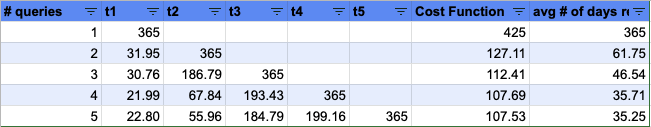
The first line is the strategy with a single query on all the data. We can see that most of the gain over the objective is done by adding a first query over 32 days of data. It makes a lot of sense as 90% of the queries are done on the previous month.

As a compromise, we chose the strategy with 3 queries, making the average number of days read per query go down from 365 days to 47 days and dividing memory usage by 7.5.

Go live and conclusion

After going live, we saw that the latency of problematic requests was divided by 2.2 in average. Even for the 99th percentile, we still got a latency decrease of 33%. It is a very good result considering:

We did not do any change to our infrastructure even though our current partitioning is clearly not good for this use case.
Even though we solved an optimization problem, changes to the code base running in production were minor and easy to understand.
As a first approximation, we divided page cache usage by 7.5 on our ClickHouse cluster for this query

Of course, we could achieve very similar results just by choosing some time ranges naively, but it is always interesting to actually understand why a strategy is working very well and when it would start to fail. Finally, it gives anyone a generic way to split any lookup query with a very big time range!

Thanks to Ryad Zenine, Sylvain Zimmer and Ali Firat Kilic for the contributions and reviewing this article. Another inspiration is The Case for Learned Index Structures, where the authors learn an index data structure using cumulative distribution function.